Tracking Potential Groundwater Plumes in Southeast Kauai

Abstract

There is often a lack of data in submarine groundwater discharge and it is often disregarded in water quality estimates, however, it plays an important role in nutrient cycling. Gathering data about submarine groundwater discharge can be useful in analyzing the conditions of coastal environments. This study focuses on using temperature and conductivity as a means of locating areas where there are potential sites for groundwater. Using Level Loggers and GPS units, data on temperature, conductivity, depth (pressure), and longitude and latitude coordinates were collected. The data was analyzed through excel and ArcGIS. The results were inconclusive possibly as a result of mixing in the ocean and problems with the data collection. Based on the data, there were places found along the coast that could be further scrutinized to see if we are actually seeing groundwater discharge in the area.

Introduction

Submarine Groundwater Discharge occurs “wherever an aquifer is hydraulically connected with the sea through permeable sediments” (Johannes 1980). SGD influences bigeochemical processes near shorelines. It is often overlooked in water quality studies, however. This study is intended to aid in identifying groundwater in the study area which stretches about 13 km from just west of Lawai Bay to Kawailoa Bay and offshore less than a kilometer. Where SGD is present, there tends to be a change in sea water chemistry, temperature, and conductivity. The focus in this particular study is the temperature and conductivity. In this climate, the temperature of groundwater tends to be lower than the seawater. Conductivity is directly correlated with the salinity of the water. Fresh groundwater has a lower conductivity than the saline sea water. Groundwater tends to be less dense than the sea water so we are focusing on the characteristics of surface water. 

Materials and methods 

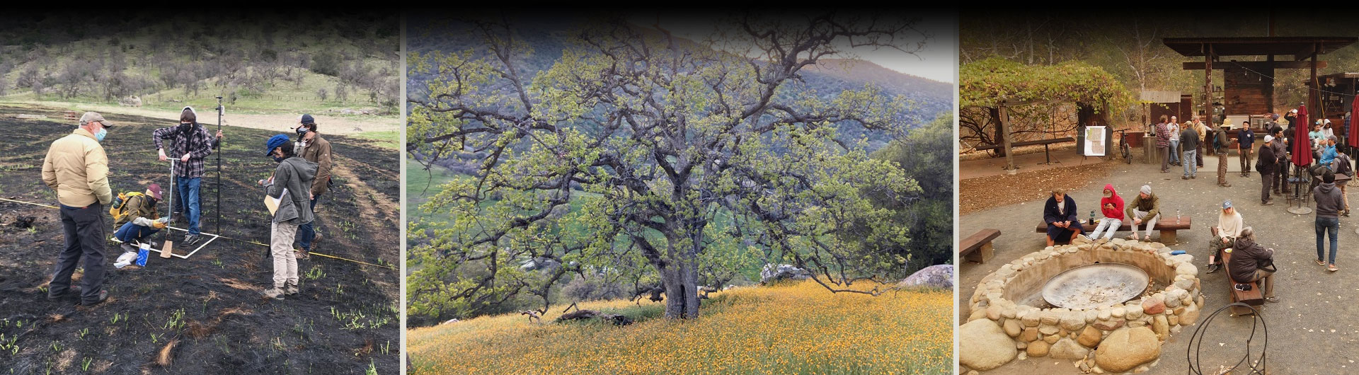
In order to identify areas where we may find groundwater plumes, we mapped out temperature and electrical conductivity levels along the Southeast coast of Kauai. Level Loggers were used to record the temperature, conductivity, and level (pressure) of the sea water. GPS units were used to record our longitude and latitude coordinates. The Level Loggers and the GPS units were synched to record the data at 5 second intervals. We transported the Loggers and GPS units by means of outrigger canoes, a fishing boat, paddling long boards, and swimming. After the data was collected, the Logger and GPS data was combined so that it could be spatially analyzed. The programs excel and ArcGIS 10 were utilized in the data analysis.

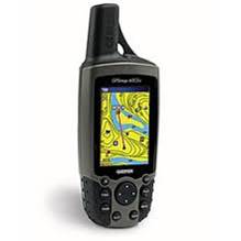
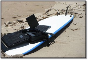
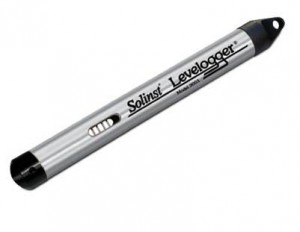
Figure 1a-1c: These figures show the type of equipment used in the field. From left to right: the Garmin (GPS unit), long board and computer, and the Level Loggers.

Results

The results generated include various maps and charts revealing information about the temperature and conductivity along the coast. The primary data used to generate these results came from the fishing boat. The reason for this is that it covers the most distance and we had the most control making sure the Loggers were in proper positioning to collect data.

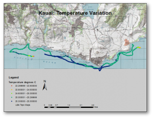
Figure 2: This figure shows the different temperatures we observed from the fishing boat. The temperature does not seem to vary much showing only about 2.3 degrees Celsius of change.

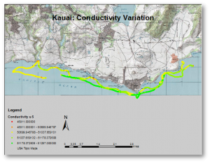
Figure 3: This figure shows conductivity change. The changes we see in conductivity seem to be by river outlets and in bays where we find freshwater. The idea is that some of this may actually be groundwater.

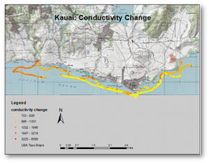
Figure 4: In this graph, I show the change in conductivity subtracting the maximum conductivity in microsiemens from the data points. Because we observed the data seem to be log normally distributed, a geometric classification was used to display the symbology. 

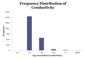
Figure 5: This figure was created to show the frequency distribution of conductivity. I normalized the data with the following equation: (Max Conductivity-Actual Conductivity)/(Max Conductivity-Min Conductivity) then took the log of the normalized conductivity. It shows that most of the water had a conductivity level indicating higher salinity levels.

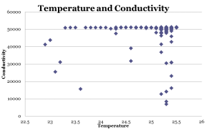
Figure 6: This figure shows that there is a lack of correlation between temperature and conductivity.

Conclusions

  In conclusion, it is very difficult, based on our data, to definitively determine where we can find groundwater plumes.  Based on the maps, a good place to start searching may be Lawai Bay. In that area, there seems to be a lower conductivity (though it may be explained by the river outlet). There was also a change in temperature, however that was very slight. It is also interesting to note that there was more conductivity change in that area. Previous studies have noted that there has been a correlation between lower temperatures and lower conductivities which would indicate the presence of groundwater, however based on our data, there was no significant correlation between the two.

  There are a lot of factors influencing temperature and conductivity. Wave and wind action may partially explain the lack of correlation. There is also solar energy that can be taken into account. The climate can cause a lot of mixing making it difficult to see conclusive results where groundwater exists. There were also some complications with the Loggers because at certain speeds, they tended to jump out of the water. In the future, it would be interesting to take a closer look and possibly utilize stronger tools to produce thermal infrared images to view the data. 

References

  Johnson, Adam G., Craig R. Glenn, William C. Burnett,   Richard N.   Peterson, and Paul G.   Lucey. “Aerial   Infrared Imaging   Reveals Large Nutrient-rich   Groundwater Inputs.”   GEOPHYSICAL RESEARCH   LETTERS  35 (2008): 13 Aug. 2008.   https://bbcsulb.desire2learn.com/d2l/lms/cont  ent/viewer/main_frame.d2l?tId=1371644&ou=  150327.

Acknowledgments

I’d like to thank Dr. Becker and Weston Ellis for all their help and organization. I’d like to thank the Outrigger team from Kauai for assisting in the data collection. I’d also like to thank Dr. Burney from the National Tropical Botanical Gardens. Also a big thanks to all those who have helped me who are associated with the GRAM program including all of the teachers, graduate students and my peers. Funding for this project was provided by the National Science Foundation.